ASCP

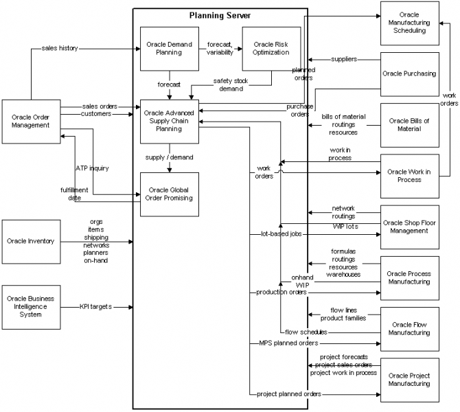
Oracle Advanced Supply Chain Planning (ASCP) is a comprehensive, Internet-based planning solution that decides when and where supplies (for example, inventory, purchase orders and work orders) should be deployed within an extended supply chain.

The key capabilities of Oracle ASCP are

Multiorganization Planning
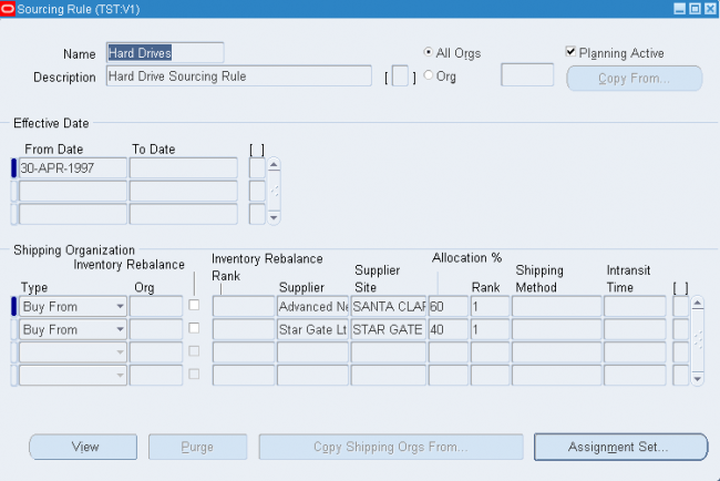
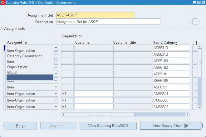
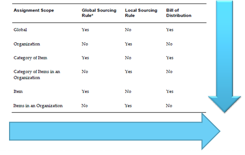
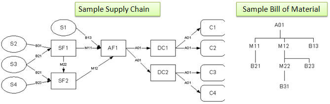
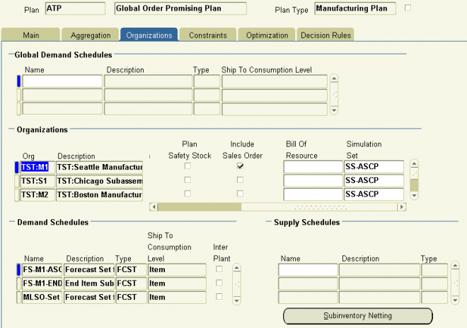
ASCP and SCP allow you to model complex supply chains and provide a unified plan for the entire supply chain. Your model can include customer preferences (for example, which organizations can supply which customers), multiple manufacturing and distribution organizations within your enterprise, and your suppliers. In simple cases, you might be able to model your supply chain using item and organization attributes. For more elaborate supply chains, you can define sourcing rules and bills of distribution and apply different sets of assignments of those rules.

Holistic Planning
The term holistic planning was coined by Oracle to suggest that one plan could meet all the needs typically addressed by multiple plans in more traditional planning scenarios. Holistic planning eliminates or reduces the need to keep multiple plans in synch. Specifically, holistic planning accommodates three dimensions of the planning problem:

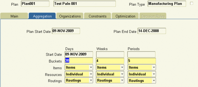
  • One plan can accommodate the entire planning horizon, with the appropriate level of granularity at different points along the horizon.
  • One plan can accommodate the entire supply chain, from your customers, through the distribution and manufacturing organizations within your enterprise, and down to your suppliers.
  • One plan can accommodate all manufacturing methods: discrete, repetitive, process, flow, and project- (or contract-) based manufacturing.
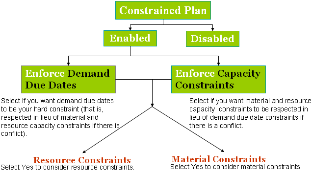
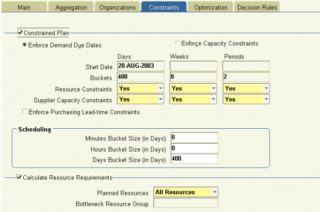
Constraints
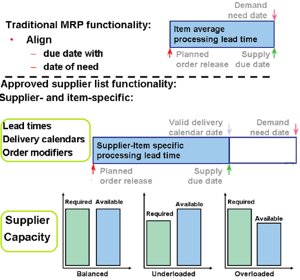
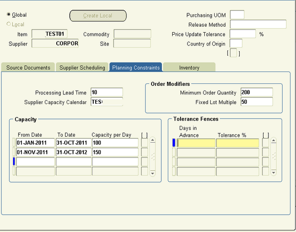
Unlike Oracle MRP planning, ASCP can respect various constraints on your production and distribution capabilities. This capability, sometimes called finite planning or constrained planning, enables you to generate a plan respecting material constraints, capacity constraints (including both manufacturing resource and transportation capacity), or both. You can plan for detailed or aggregate resources, and you can use item routings or bills of resource to control the granularity of the planning process.

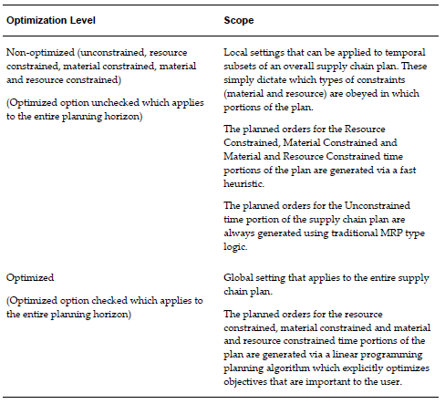
You can enforce constraints selectively across the planning horizon. It may be important, for example, to recognize material and capacity constraints in the near term to avoid creating a plan that you can’t execute. But at the far end of the horizon, it may be more important to generate an unconstrained plan to determine how much additional capacity you might need to meet the anticipated demand.

Constraint-based planning is a prerequisite for optimized planning—if there are no constraints, the assumption is that you can do anything; there’s nothing to optimize.
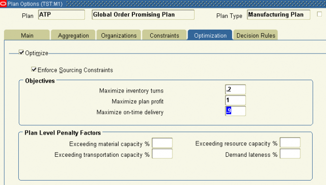
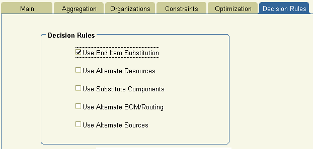
Optimization
ASCP includes the option to generate an optimized plan. In an optimized plan, the planning process determines the relative cost of the different options available to it and chooses the “best” alternative based on those costs. Some of those costs are naturally present in your ERP data, such as the cost of using a substitute item or an alternate resource. Other costs are computed in planning by applying penalty factors to different events. For example, you might assign a penalty factor of 50 percent to exceeding resource capacity (reflecting that you would pay time-and-a-half if you had to work overtime); you might assign another penalty factor to satisfying a late demand, to artificially add cost to late production. In addition, optimization is influenced by the weight you give to each of three explicit planning objectives: Maximize Plan Profit, Maximize On-Time Delivery, and Maximize Inventory Turns.
 

Integrated Performance Management
ASCP incorporates performance management features from Oracle’s Business Intelligence System (BIS). The Planner Workbench for ASCP displays four Key Performance Indicators (KPIs) for each plan:

  • Inventory Turns The inventory turns you could achieve if you executed the plan as suggested
  • On-Time Delivery The percentage of ontime delivery, to customer orders or to internal orders, that the plan projects
  • Margin Percentage The anticipated margin (profit) that would be generated by following the suggestions of the plan
  • Resource Utilization The utilization of resources projected by the plan

Release 11i.5 ASCP provides additional KPIs; right-click the workbench to select the following indicators:

  1. Margin The margin amount (i.e., currency) that would be generated by following the plan suggestions
  2. Cost Breakdown A comparison of four separate costs—Production Cost, Inventory Carrying Cost, Penalty Cost, and Purchasing Cost
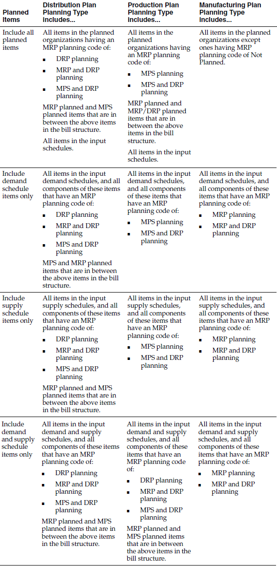
You can use BIS to define targets for each of these KPIs. The Planner Workbench displays a graph for each of these KPIs and their targets so that you can easily assess the effectiveness of a particular planning strategy. ASCP also provides enhanced exception messages and uses Oracle Workflow to provide notification and response processing for all those exceptions.

Plan Types
ASCP uses basically the same plan types as traditional MRP, but uses slightly different names:

  • Distribution Plan equates to a DRP, or Distribution Requirements Plan.
  • Manufacturing Plan equates to an MRP, or Material Requirements Plan.
  • Production Plan equates to a Master Production Schedule, although there are significant differences between the earlier MPS and a Production Plan defined in ASCP. 
Architecture

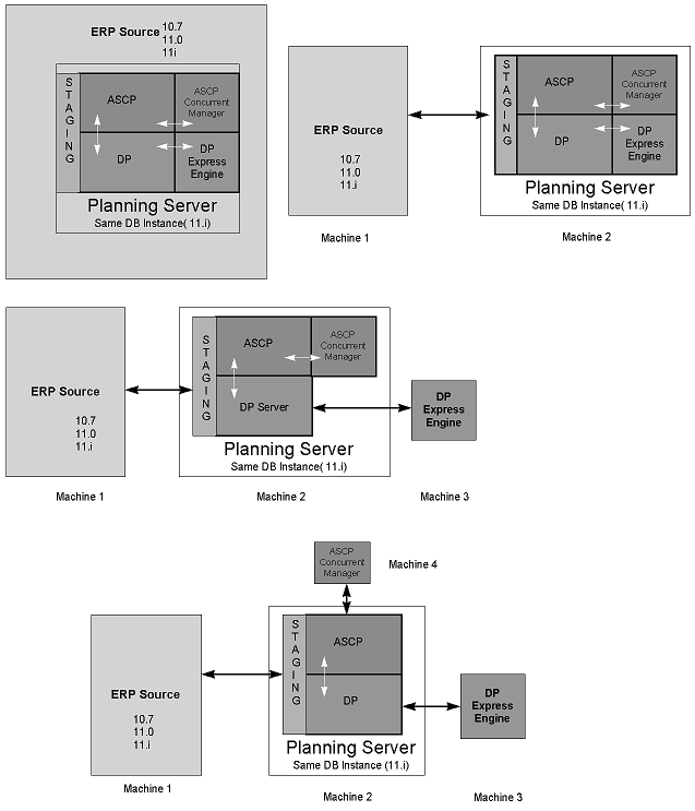
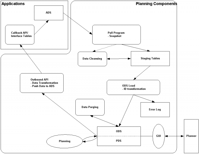
ASCP is able to run on a separate server from your ERP system. This architecture eliminates any performance degradation on your transactions systems when a plan is running, and it enables you to run plans more often and more quickly than with traditional planning systems. (If you will run your plans overnight or at nonpeak hours, you can use the same server for both ASCP and ERP.)

The separate-server architecture also facilitates planning for multiple ERP systems; you can define multiple ERP instances to plan, collect their data to the planning server, and then run one single, consolidated plan with the aggregate data.

Because planning is designed to run on a separate server from ERP, you must explicitly publish the planning data back to the source instance to perform certain activities in your ERP system. The Push Plan Information concurrent program provides this function. For example, if you want to create flow schedules from an ASCP plan, you must run this program.

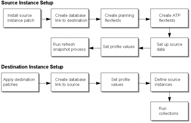
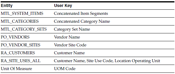
Whether you run ASCP on a separate machine, a single machine, or the same database instance as your ERP system, the process of setting up and running ASCP plans is unchanged—you must still define the source instances that planning will use and you must still collect data from those instances to the planning server.
 

Multiple Sourcing Options

Oracle provides sourcing rules and bills of distribution to model multiple sources, including splitting production or purchases across plants or suppliers. These sourcing rules and bills of distribution are assigned to items, organizations, or categories using Assignment Sets.
Both sourcing rules and bills of distribution use effectivity dates to let you project changes to your supply chain over time. The effectivity date initially defaults to the system date; like effectivity dates in routings or bills of material, a “null” ending date means that the effectivity of the rule has no projected end.

1. For each effectivity range, you define the sourcing options associated with the rule. There are three possibilities:

Make At This option specifies that you will make any items associated with the rule at the receiving organization.

Buy From This option indicates that you will buy any items associated with the rule from a specified supplier. With the Buy From option, you must enter the appropriate supplier, and optionally, the supplier site.

Transfer From This option specifies a different organization within your enterprise as the source of items associated with this rule. With the Transfer From option, you identify the source organization; you must have already defined the shipping network between the source and receiving organization. You can also select a ship method from the shipping methods you defined in your shipping network; this will determine the in-transit time and shipping cost, which planning will use in its calculations.

2. Though the mechanics of defining sourcing rules and bills of distribution are much the same whether you’re running ASCP or SCP, they operate very differently based on your planning method and options.

For ASCP, you assign each option a priority code/Rank. A priority code serves as a method for defining multiple sourcing scenarios—all the options within a single priority code will be considered as a unit. Within a priority code, you assign a percentage to each sourcing option. For example, if you have a group of items that you plan to buy from two different suppliers, you might define a sourcing rule with two “buy from” options within the same priority, specifying 50 percent for each supplier. If an alternate scenario for the same set of items is to buy from a single supplier, you would define a second scenario (priority) within the same sourcing rule, assigning the single supplier 100 percent of the purchases. Within a single priority code, the percentages must total 100 percent, or the group of options will not be considered by planning.

For SCP, the entire rule is treated as a single scenario; each option typically has a different priority code, which is used to “break a tie” if two options have identical planning percentages

You can define sourcing rules, bills of distribution, and assignment sets in your ERP instances; they will be collected with other planning data in the data collection process. This approach makes sense if you have only one source instance, or if you want to use the same sourcing rules for other functions within your purchasing system. For example, you may want to use the same sourcing rules in your supplier item catalog that you use for planning.
You can also define sourcing rules, bills of distribution, and assignment sets on the planning server itself; this approach is useful if you will be planning for data collected from multiple ERP instances.

3. Sourcing and Assignment APIs
Oracle provides two APIs to create sourcing information—the Sourcing Rules/Bill of Distribution API and the Sourcing Rules/Bill of Distribution Assignment API. Their use is described in the Oracle ASCP and Global Order Promising Technical Reference Manual, available as part of the Oracle documentation library.
 

Sourcing Rules

You can define sourcing rules that specify how to replenish items in an organization, such as purchased items in plants. Sourcing rules can also specify how to replenish all organizations, as when the entire enterprise gets a subassembly from a particular organization.

If there is a conflict between a sourcing rule and a bill of distribution, the sourcing rule takes precedence.


1.1. Enter a unique sourcing rule name.

1.2. Indicate whether this sourcing rule is used for all organizations (global) or a single organization (local). If the sourcing rule is local, you must enter an organization name; otherwise, your current organization will be the receiving organization.
Here global means accross OUs. The same sourcing rule can be used in a differnt OU. If you make the sourcing rule as global then while selecting the supplier site we can choose a site from a differnt OU.

1.3. Choose Copy From to copy the effectivity dates and shipping organization from another sourcing rule into this one.

2.1. Enter effectivity dates. You must enter a start date, but entering an end date is optional.
For each range of effectivity dates, you can include multiple shipping organizations.
For each shipping organization you want to include, select a sourcing type to specify whether you make, buy, or internally transfer the item. You can also copy a list of shipping organizations from an existing sourcing rule. If you enter a customer organization as the receiving organization, then you cannot select a supplier organization as the shipping organization.

3.1. Enter an allocation percentage for each shipping organization. Allocation percentage includes the number of planned orders issued to the part for the entire the planning horizon. Your total allocation may not exceed 100. If the allocation percentage for all the shipping organizations included within a range of effectivity dates equals 100, Planning Active is checked. If the sourcing rule is not planning active, the planning process will not use the rule to assign planned orders.

3.2. Enter a numeric rank value to prioritize each sourcing type. If you have two sources with the same allocation percentage, planned orders are sourced from the highest rank first.

3.3. Select a shipping method, such as FEDEX, UPS, or rail


Bills of Distribution

You can define bills of distribution that specify a multilevel replenishment network of warehouses, distribution centers, manufacturing centers (plants), and trading partners.

 
1.1 Enter a unique bill of distribution name.
1.2. If the allocation percentage for this bill of distribution equals 100, Planning Active is checked.
Note: You cannot set the allocation percentage to less than or greater than 100 for sourcing rules that are already assigned in assignment sets
1.3. Choose Copy From to copy the receiving and shipping organization information from another bill of distribution into this one.
2.1. Enter the effectivity dates for each receiving organization in this bill of distribution.
3.1. For each receiving organization, you can enter a number of shipping organizations.
For each shipping organization, select a sourcing type to specify whether you make, buy, or internally transfer the item. You can also copy a list of shipping organizations from an existing bill of distribution.
Note: Suppliers and supplier sites must be predefined in Oracle Payables.
3.2. Enter an allocation percentage for each shipping organization. Allocation percentage includes the number of planned orders issued to the part for the entire the planning horizon. Your total allocation may not exceed 100. If the allocation percentage for all the shipping organizations included within a range of effectivity dates equals 100, Planning Active is checked. If the sourcing rule is not planning active, the planning process will use the rule to assign planned orders.
Note: For bills of distribution that are already named in assignment sets, you cannot set the allocation percentage to less than or greater than 10
3.3. Enter a numeric rank value to prioritize each sourcing type. If you have two sources with the same allocation percentage, planned orders are sourced in rank order.
3.4. Select a shipping method, such as FEDEX, UPS, or rail
 

Assignment Sets

Once you have defined your sourcing rules and bills of distribution, you must assign them to particular items and/or organizations. These assignments are grouped together in assignment sets. This is where your various sourcing strategies define a particular supply chain network.

Each assignment set to represents selection of organizations and/or items you want planned. To influence the planning process, you must include an assignment set in your plan options.

In an assignment set can assign your sourcing rules and bills of distribution at different levels, as follows:

  1. Global
  2. Organizations
  3. Categories
  4. Categories Organizations
  5. Item
  6. Items Organizations

These levels allow you to assign a replenishment rule to as many or as few items as possible. For example, a category of items could be defined as packaging material, and a sourcing rule that identifies the suppliers could be assigned.
 

1.1. Enter an assignment set name and description.
Note: The assignment specified in profile option MRP: Default Sourcing Assignment Set is the only one used by Oracle Purchasing for its processing

2.1. Select an Assigned To type.
Note: You can assign a sourcing rule or bill of distribution to a category only if you have updated the profile option MRP:Sourcing Rule Category Set. See: MRP:Sourcing Rule Category Set

2.2. Enter an organization name, if the Assigned To type requires one.
Note: You cannot assign customers modelled as organizations to a global sourcing rule

2.3. Enter the name of the customer to which you want to assign a sourcing rule or bill of distribution.

2.4. Enter the specific site to which you want to assign a sourcing rule or bill of distribution.

2.5. Enter an Item/Category if you selected Item or Item-Org as the Assign To type.

2.6. Enter the sourcing rule or bill of distribution as the Type.

2.7. Enter the name of the sourcing rule or bill of distribution.

Assignments Hierarchy
In the following table, rows below override rows above them. Columns on the right override columns on the left.

Notes
1. After defining the soucing rule and assignment set one needs to enter the default asignment to be used in the profile option MRP:Default Sourcing Assignment Set.

Choosing Plan Classes

A big difference between ASCP and earlier planning methods is the option of planning to constraints. Although Oracle has supported simultaneous material and capacity planning for a long time, the planning engine has always planned to meet due dates; capacity planning has been unconstrained, or infinite. ASCP provides the option of constraint-based planning, or finite capacity planning.

Furthermore, you can choose to plan to capacity (including transportation capacity) constraints, material constraints (including modeling the capacity of suppliers to provide material), or both; and you can specify different constraints and different levels of granularity in the different periods of the planning horizon.

Oracle ASCP allows for the following options for generating plans.

  1. Unconstrained
  2. Resource Constrained
  3. Material Constrained
  4. Material and Resource Constrained
  5. Optimized
Before discussing these options in the table below, please take note of the following key concepts.
Constraints
Oracle ASCP lets you prioritize how you enforce Capacity Constraints or Demand Due Dates. Whichever constraint takes precedence over the other is the hard constraint; the other is the soft constraint. You must choose one and only one type of constraint.

Enforce Demand Due Dates
If you choose to enforce Demand Due Dates (setting Demand Due Dates as a hard constraint), then primary resources are used and loaded to capacity to satisfy demand due dates. The system also evaluates alternate resources if additional capacity is required. If there is insufficient capacity to meet demand due dates, the primary resource is overloaded. The choice of whether to use an alternate resource or overload capacity depends on cost considerations if optimization is selected. Oracle ASCP returns exception messages if capacity is overloaded.

Enforce Capacity Constraints
If you choose to enforce Capacity Constraints (setting Capacity Constraints as a hard constraint), then resources are loaded to their limit to satisfy demand (if required). Unsatisfied demand is pushed into the future. In this case, Oracle ASCP returns late replenishment exception messages.

Optimization
Oracle ASCP allows for multiple levels of optimization in generating plans. These are described in the table below along with the situations under which each would be most useful.
 
The scope of optimization levels is summarized in the table below:


Planning Business Flows

This section describes the flows of information between the components of the Oracle Advanced Planning Suite and provides an overview of how these components are to be used together in order to accomplish several key business flows.
Topics covered in this section include the following:

  • APS Information Flows
  • The Demand-to-Make / Demand-to-Buy Business Flow
  • The Inquiry-to-Order Business Flow
APS Information Flows
The major information flows between the components of the Oracle Advanced Planning Suite and the rest of Oracle Applications are shown in the figure below.
The Demand-to-Make / Demand-to-Buy Business Flow
The demand-to-make /demand-to-buy business flow begins with the establishment of independent demands that will drive the activities of the supply chain. On the basis of sales history from Oracle Order Management, Oracle Demand Planning generates statistical demand forecasts. After adjustment by planners, these forecasts and
their variability as estimated by Oracle Demand Planning are then input into Oracle Inventory Optimization.

Using user-supplied information about the variability of this forecast demand and the variability of supplier lead-times, Oracle Inventory Optimization generates an optimal time-phased safety stock plan.

Oracle Advanced Supply Chain Planning (hereafter, Oracle ASCP) considers three streams of independent demand: the safety stock planned demand from Oracle Inventory Optimization, forecasts from Oracle Demand Planning, and sales order demand from Oracle Order Management. Oracle ASCP outputs a time-phased supply plan (planned orders) that can then be released directly to the appropriate execution systems: Oracle Purchasing, Oracle Work in Process (for discrete manufacturing), Oracle Process Manufacturing, Oracle Flow Manufacturing, Oracle Project Manufacturing, or Oracle Shop Floor Management (for semiconductor manufacturing).

The Inquiry-to-Order Business Flow
The demand/supply picture output by Oracle ASCP serves as the basis for the order promising results calculated by Oracle Global Order Promising. Oracle Global Order Promising can be called either from a customer-facing order capture application such as a web store or from Oracle Order Management.

In the inquiry-to-order business flow, an inquiry for a potential order is sent from Oracle Order Management to Oracle Global Order Promising. The fulfillment date returned by Global Order Promising, if later than the original request date, is populated as the new request date of the order. This request date validation process is called scheduling. Once an order is successfully scheduled, then it can be booked and made visible to Oracle ASCP for supply planning purposes.

Planning Cycle
This section describes an end-to-end planning flow that a planner might perform during the course of a planning cycle. The flow demonstrates the key features of Oracle ASCP that a typical planner would use in the course of their work. The general flow that occurs during a planning cycle is shown in the figure below.

ASCP Setup

Oracle Advanced Planning Suite has a component architecture that separates the transaction data and associated processing (for example, inventory receipts and order entry) in a source instance from the planning calculations done in a destination instance. This allows planning calculations to be done on a different physical machine
than the machine that performs transactions and results in better system response. It also allows planning calculations (demand planning, inventory planning, supply planning and order promising) to be applied simultaneously to information from across multiple source instances, which is useful when transaction information for a global supply chain is spread across multiple instances. Oracle Demand Planning also uses athird instance, an Express database, to hold data while multidimensional manipulation of demand data occurs.

The source can be any ERP system, but out-of-the-box integration to the Oracle Advanced Planning Suite destination instance (planning server) exists in some cases but not in all cases.

Set up for Oracle Advanced Planning Suite consists of steps for the source, steps for the destination, and steps for Express.

APS may be implemented in two possible configurations:
Centralized Planning
A centralized configuration implies that the ERP applications and APS share the same Oracle instance on one server.
Decentralized Planning
A decentralized configuration implies that the ERP applications and APS are executing within two separate Oracle instances, possibly on the same server.

  • Both configurations are supported using a consistent architecture with the sole distinction being that the decentralized configuration requires the use of database links to pull data into the MSC data store
  • APS nomenclature employs Source and Destination when speaking of the ERP transaction data store and the planning data.  Data, at the source, is collected into the destination or operational datastore (ODS) where planning activities occur. If a centralized configuration is implemented, both the source and destination are operating within the same Oracle instance. 
In Oracle Advanced Planning, transaction processing and planning occur in separate database instances, the source instance and the destination instance. If you deploy any Oracle Advanced Planning module using this multi-instance configuration, please note the important restriction that both source and destination database instances must be on the same major release of the Oracle database; either both instances must be on Oracle 8i or both instances must be on Oracle 9i. The configuration source on 8i with destination on 9i is not supported and the configuration source on 9i with destination on 8i is not supported.
The following figure is a flowchart illustrating the source and destination setup steps.

Multti-Machine Implementation


For small implementations, source, destination, and Express can reside on the same machine and be in the same instance.

For larger implementations where system throughput is more important, the various instances can be deployed on separate machines. A two-machine deployment configuration is appropriate when the size of the demand planning data is relatively small.

A three-machine deployment allows for the manipulation of high-dimensionality, large-scale demand planning data to occur on a machine separate from the planning calculations done on the planning server. The following figure illustrates this configuration.

The Advanced Supply Chain Planning concurrent manager may also be deployed on a separate machine.

Setup Flowchart

 
 Implementing APS in centralized mode is only possible when collecting from an 11i source.A centralized implementation does not require database links.  Since the planning flexfields are included in 11i, submitting the concurrent process, Create Planning Flexfields is not required.  All other setup discussed in this document are required.

Running Collections

Oracle ASCP has a component architecture that allows a single instance of Oracle ASCP to plan one or more transaction instances. The transaction instances can be a mixture of releases. The Oracle ASCP planning instance (referred to as the planning server) can sit on the same instance as one of the transaction instances, or be a separate instance altogether. In either case (even if the planning server shares an instance with the transaction instance to be planned), data to be planned is brought from the transaction instance(s) to the planning server via a process called Collection.

Oracle ASCP uses a data store based on the planning data model that is exposed through interface tables. The data is pulled from the designated data sources into its data store; Oracle ASCP Collections are responsible for synchronization as changes are made to the data sources.

The configurability of the collections is enabled through a pull program based on AOL concurrent program architecture. Thus, for example, different business objects can be collected at different frequencies. Supplies and demands, which change frequently, can be collected frequently. Routings and resources, which change relatively less often, can be collected less frequently.

Standard collections process: Using the standard collections process, you can manually run three types of collection methods including a complete refresh, a net change refresh, or a targeted refresh on specific business entities.

Continuous collections process: The continuous collections process is an automated process of data collection that efficiently synchronizes the data on the planning server by looking up the sources. If you opt for continuous collections, the system
automatically determine the type of collection that needs to be run on entities selected by you. The continuous collections process collects data from the sources with the least user intervention. The Continuous Collections concurrent program
performs continuous collections.

Definitions:
You should be familiar with the following terms before examining the data collections architecture:
Applications Data Store (ADS): The set of source data tables in each transaction instance that contain data relevant to planning.
Data Pull: The data collection process consists of the Data Pull and the Operational Data Store (ODS) Load. The collection process lets you collect across several Oracle  aplication versions. It supports several configurations. The two types of collections process are standard and continuous.
Operational Data Store (ODS): The planning data tables in the planning server that act as destination for the collected data from each of the data sources (both ADS and Legacy).
Planning Data Store (PDS): The outputs of the planning process. The PDS resides in the same data tables as the ODS. However, PDS data are marked with plan IDs that show which plans they correspond to, while ODS data are marked with plan ID = -1.
Collection Workbench: The Collection Workbench is a user interface for viewing data collected over to the planning server from the transaction instances. The functionality here is similar to Planner Workbench functionality. For more information on the Planner Workbench

Standard Data Collection: The standard data collection process enables you to select the mode of data collection from a complete refresh, an incremental refresh, or a targeted refresh.
Standard data collection consists of the following processes:

  • Pull program: Collects the data from the ADS and stores the data into the staging tables. This pull program is a registered AOL concurrent program that could be scheduled and launched by a system administrator. If you are using a legacy program, you must write your own pull program.
  • ODS Load: A PL/SQL program which performs the data transform and moves the data from the staging tables to the ODS. This collection program is a registered AOL concurrent program that could be scheduled and launched by the system administrator.
Continuous Data Collection: The continuous data collection process automates the process of looking up the sources to populate the tables on the planning server. With the least user intervention, the continuous data collection process determines the type of collection to perform on each type of entity. The Continuous Collections concurrent process performs continuous collections.

Defining Supply Chain Plans

Oracle ASCP can generate planned orders for an entire supply chain within a single multi-organization supply chain plan. This is illustrated below with a sample supply chain;  and'Sample Bill of Material.

 
In this sample supply chain, SF1 and SF2 are subassembly facilities, AF1 is a final assembly facility, DC1 and DC2 are distribution centers, C1, C2, C3 and C4 are customers and S1, S2, S3 and S4 are suppliers. A single plan of the entire supply chain has the following inputs:
  • Demand quantity (forecast + actual sales orders) for A01 at DC1 for each of the time buckets in the planning horizon. This is captured in a Master Demand Schedule (MDS) for DC1.
  • Demand quantity for A01 at DC2 for each of the time buckets in the planning horizon. This is captured in an MDS for DC2.
  • The plan output contains planned order quantities, start dates, and completion dates for A01 and all of its components and subcomponents.
Prerequisites for Running a Global Supply Chain Plan
To run a global supply chain plan, the following prerequisites are required:
  • Each planned organization must be set up on the source instance.
  • Collection programs must be directed to collect data from the transactional instance of each planned organization.
  • Items to be planned must be enabled in each organization that can produce (or distribute) the item. During item setup, items can be enabled in all organizations or only in specific organizations.
  • Routings and/or Bills of Resource for each planned item must exist or be enabled in each organization that is planned centrally.
  • Suppliers and sourcing rules must be enabled in all relevant organizations.
Advantages of the Single Plan
The single-plan approach is advantageous for the following reasons:
  • Least planning effort: Fewer plans need to be generated; fewer planning servers need to be deployed and maintained.
  • Data consistency: Without the single-plan ability, requirements must be repeatedly transferred upstream within the supply chain to each successive supplier facility.Each transfer presents an opportunity for miscommunication or data loss.
  • Global optimization: Intelligent trade-offs between the performance of individual facilities (as measured by, for example, plan profit) can be made because Oracle ASCP optimizes the supply chain planned orders as a whole.
  • Minimum communication lag:The effects of decisions made at the highest level of the supply chain are immediately visible at the lowest level of the supply chain. If individual facility plans are used, there is at least a one planning-run duration lag between the receipt of requirements at a facility and the passing of the dependent requirements to the facility's suppliers. Moreover, this lag is often much greater due to differences in working hours between upstream and downstream facilities (for example, if the facilities are in different time zones). Also, the planning cycles of upstream and downstream facilities may not be synchronized (for example, customer facility AF1 runs its plan on Monday, while supplier facility SF1 runs its plan on Sunday). This results in even longer communication lags. The overall effect of plan communication lag is to make the supply chain less responsive to meeting changes in customer demand
 

Creating Supply Chain Plans

You can have multiple supply chain plans. Before you launch a plan for the first time you must name it.
Copying Supply Chain Plans
In addition to creating a plans by creation, you can create a new plan by copying information from one plan to it. Do this if you want to:

  • Save the results of a particular plan run before you re-run the plan
  • Begin using a new plan name with the results of the latest run of another plan.
  • Create a new plan with the same plan options as an existing plan
Use the copy plan function to make a copy of an existing plan. If memory bases planner flat files do not exist, Copy Plan process completes with the warning - WARNING: The copy plan operation completed successfully. However, some auxiliary data files could not be copied. Therefore, you will not be able to run online planner. You can re-launch the plan from the Navigator.

Create a global supply chain plan

Navigator to Supply Chain Plan > Names
Enter the below details as required
Name: Define a plan name.
Description: Define a plan description.
ATP:  If this is selected, this plan will be used for availability check. If the plan is used as a 24 x 7 ATP plan, the planning process may never switch to a new version of the plan from the copied plan after the original plan has completed successfully ; consider setting profile options MSC: Action Allowed on ATP 24 x 7 Plan While Running and MSC: ATP  Synchronization Downtime (minutes).
Production: If this is selected, this is a product plan. Planned orders will be automatically released within their release time fence.
Notifications: If this is selected, exception message notifications for the plan are enabled.
Plan Type Valid values are Manufacturing Plan, Production Plan, and Distribution Plan. This setting interacts with the Planning Method item attribute to determine which subset of the items that pass the condition imposed by the Planned Items parameter are planned.

Choosing a Plan Type
In Oracle ASCP you can launch three type of plans:
  •  Production Plan
  •  Manufacturing Plan
  •  Distribution Plan
Each creates time-phased planned orders that satisfy independent and dependent demand while seeking to respect material and resource constraints. A choice of plan types lets you tailor the degree of subset planning that is performed for the supply chain: from a single, global supply chain plan down to manually adjusted plans for each item in each organization of the supply chain.

MPS plans support the following functionality:
  •  You can select routings for a production plan while scheduling resources.
  •  For production plans that have routings, you can view the Gantt chart in the Planner Workbench.
To do this, the three types of plans need to be used in conjunction with the MRP Planning Type item attribute that is set for each item. Possible values for this attribute are:
  • MRP Planning
  • MPS Planning
  • MRP/DRP Planned
  • MPS/DRP Planned
  • DRP Planned
The below table lists the controls that determine the items that are planned in the plan and their possible values:

Planning Business Flows

Collection Strategy

Major features of the collection process include:
Multiple Source Instances
You can register any number of source data instances and non-Oracle data sources on each Oracle ASCP installation.

Pull Architecture
You can collect new source data instances into Oracle ASCP with minimal impact. The data is pulled from the source data instance by Oracle ASCP. Each instance can have its own refresh interval. A failure in one instance will not affect data collections from other instances.

Detect Net Change to Synchronize Oracle Applications and Oracle ASCP
You can synchronize the data in Oracle Applications transaction instances and the Oracle ASCP planning server in a net change mode. Thus, only the changed source data is collected each time, reducing the computational burden on the collection process.

Multi-Process Collection Architecture
You can enhance the performance of the pull program by distributing the tasks to multiple collection workers.

Data Consolidation
The collection program can consolidate the entities shown in the following table across instances based on the corresponding user-defined keys. For all the entities not described in the table, the instance ID together with the entity key in each instance uniquely identifies each row.


Projects/Tasks, and Seiban Numbers
You can consider Projects, Tasks, and Seiban Numbers to be unique within the context of an Oracle Applications instance; no consolidation is required.

Support for Several Configurations
You can perform centralized and decentralized configurations based on the scale of the enterprise and specific business needs. Source data applications and Oracle ASCP can reside on one server or on separate servers.

Architecture
Oracle ASCP’s data collection architecture, shown in the figure below, depicts the data objects, procedures, and data flow between source data and Oracle ASCP. The major repositories are ADS, ODS, and PDS. Procedures enable data cleansing, data collecting, data communication, and net-change handling between data repositories.

When Oracle ASCP and its source data reside on the same instance, communication between them is enabled by PL/SQL based public API procedures or interface tables. In a distributed environment, procedure calls are made using database links.


Collection Methods

Collecting data can take a significant amount of time compared to the time for the overall planning cycle. Oracle Advanced Supply Chain Planning (ASCP) provides a collection method that allows the collections duration to be reduced in cases where information about some - but not all - planning-related business entities on the planning server needs to be updated.

There are three collection methods:
■ The Complete Refresh method clears all transaction data for all business entities from the planning server (for the source instance being collected), then copies over information about the user-selected entities. This method can be time consuming.
■ The Targeted Refresh method clears transaction data for only the user-selected business entities from the planning server, and then copies the entity information over from the transaction instance. Information about nonselected entities remains intact on the planning server. All planning business entities are supported by Targeted Refresh collections.
■ The Net Change Refresh method copies only incremental changes to business entities to the planning server (and is thus faster), but is supported mainly for demand and supply business entities only.

When To Use Each Collection Method
You should use Complete Refresh the first time you perform collections from a source instance to the planning server. You may also wish to use complete refresh collections after a significant proportion of the setup data in your transaction system has been altered, and you would like to make a fresh copy of all source instance business entities (items, bills of material, sourcing rules, resources, and so on) on the planning server. You typically collect all business entities in a Complete Refresh Collection.

You should use Net Change Refresh if you would like to update the supply and demand picture on the planning server as quickly as possible, and the incremental changes to supply and demand in the source instance since the last collection have not been extensive relative to the existing (already collected) body of supply and demand information. In this case, Net Change Refresh is the fastest way to achieve the desired update of the planning server operational data store, because it copies over from the source instance only the incremental changes in supply and demand since the last collection.

You should use Targeted Refresh if you would like to update the planning server information for some (but not all) business entities, and some of these entities fall outside the category of supply and demand entities supported by Net Change Refresh. For example, to update the planning server with a newly rebuilt manufacturing calendar, you would run Targeted Refresh collections for just the
calendar business entity. Data on the planning server about all other business entities would remain unaffected by this collection.

You would also use Targeted Refresh (in lieu of Net Change Refresh) to bring over the latest picture of supply and demand to the planning server in cases when the incremental changes to supply and demand on the source instance since the last collection are very extensive. In this case, the update mechanism employed by Targeted Refresh collections (wholesale deletion followed by rebuilding of data on the planning server) is faster than the mechanism employed by Net Change Refresh collections (incremental insertions into existing data on the planning server).

If you want the mode of data collection to be determined by the system, select Continuous Collections.

Subset Plans

There are some situations in which it makes sense to plan a portion of the supply chain separately, outside of the overall supply chain DRP plan.


Scenario 1: Unique Local Objectives Must be Respected Along with Global Objectives Suppose that subassembly plant SF1 (Figure 5–1, “Sample Supply Chain”), which makes M12 (Figure 5–2, “Sample Bill of Material”), contains very expensive capital equipment. SF1 is the overall supply chain constraint, so every minute that its resources are utilized brings extra profits to the enterprise. Resource utilization is the most important objective for SF1. For the supply chain as a whole, however, due to rapid product life cycles and a fickle market, inventory turns might be the most important objective. In this situation you could run a two-stage
planning process.
  • An MRP for organization SF1 with resource utilization as the objective to generate planned orders for M11, M22, B31, and B21 (the portion required at SF1).
  • A DRP for organizations DC1, DC2, AF1, SF1, and SF2 with the above MRP as a supply schedule with inventory turns as the objective to generate planned orders for A01, M12, B13, B23, and B21 (the portion required at SF2).

Scenario 2: Local Restrictions Not Captured in Global Planning Inputs Suppose that item B21, a subcomponent of item M11 (Figure 5–2, “Sample Bill of Material”), has volatile pricing. In lieu of implementing the default planned orders in facility SF1 that a global DRP would generate for M11 and its subcomponents (B21), one could plan the supply chain as follows:
1. DRP plan for organizations DC1, DC2, AF1, and SF2 to generate planned orders for A01, M12, B13, M22, and M11.
2. Load the DRP as a demand schedule into a Master Production Schedule (MPS) for organization SF1. Dependent demand for M11 is derived from the planned orders for A01.
3. Run the MPS.
4. Manually adjust the planned orders for M11 in the MPS (for example, to pull ahead the orders for M11 in order to take advantage of a time-sensitive special promotion on B21.)
5. Run an MRP for organization SF1 with the adjusted MPS as input to create planned orders for M11 components and  subcomponents (B21 in this case).

Situation 3: Single Global Data Model Not Available The one-step supply chain planning capability of Oracle ASCP presumes either the installation of ASCP as part of an enterprise-wide implementation of Oracle Applications, or the existence of collection programs to pull cross-supply chain transaction data from various Oracle Applications instances or from legacy systems. Cross-supply chain data must be accessible to build the net change snapshot used by Oracle ASCP to generate planned orders.

This may not be the case. For example, one or more facilities in the supply chain perform planning and/or transaction processing on legacy systems not yet integrated to Oracle ASCP via some sort of collection program. In this situation, the renegade facilities must be scheduled outside the global DRP plan according to the same steps as used in Scenario 2 above.

Pitfalls of Subset Planning
The two principal pitfalls of subset planning (as opposed to global, single-plan supply chain planning) are:
  • local optimization as opposed to global optimization
  • plan infeasibility due to supply chain interdependencies
The first pitfall is the fact that plans that optimize individual facilities may not be compatible with the optimum global supply chain plan. Take the case of the two distribution centers DC1 and DC2 in Figure 5–1, “Sample Supply Chain.” The way to maximize ontime delivery for DC1 is to allocate all production from AF1 to DC1.

The same logic holds for DC2. The global optimum solution, which would be missed via subset planning, comes from some allocation of AF1 output to both DC1 and DC2. A simple example of supply chain interdependency is Supplier S3 in Figure 5–1, “Sample Supply Chain.” This supplier supplies item B21 to both subassembly facilities SF1and SF2. Individual plans run for SF1 and SF2 could not recognize the shared capacity at supplier S3 and could not evaluate, if the combined SF1 and SF2 demands for B21 are too high, how best to allocate the B21 to SF1 and SF2. In such a situation the SF1 and SF2 individual plans would be infeasible, but would not even generate any exception notices to alert the planners.

Choosing Between Global Supply Chain and Subset Plans
In general, resource and material capacity are most efficiently utilized in a global supply chain planning environment where planning distributes production requirements across multiple organizations. However, the choice of global supply chain versus subset planning should depend on a number of factors including:
■ Physical proximity of the organizations being planned – If planned organizations are geographically dispersed, it is generally more difficult to fulfill demand in one region from a plant or distribution center far away because of transportation costs and longer lead times. Note, however, that the costs associated with fulfilling demand from remote plants can be modeled in planning. Planning can then optimize production allocation across plants to meet the objectives that have been set. For example, if balancing resource loads
is the primary objective of a multi-organization plan, planning will distribute production across plants to meet that objective.
■ Commonality of the items produced – If you have multiple organizations that produce similar products, global supply chain planning is beneficial because planning can consider factors like material and resource availability, material costs, and resource costs to create an optimal supply chain plan.
■ Commonality of the supply base –Similar to producing common items, organizations sharing suppliers are good candidates for global supply chain planning because supply can be optimally distributed across plants depending on each plan’s production requirements. Global supply chain planning will ensure that supplier capacity is most effectively used to meet end customer demand and to minimize inventory.
■ Linkage among plants – If production at one plant must be coordinated with production at other plants, global supply chain planning should be used. For example, if Plant A provides subassemblies to Plant B (Plant A is a feeder plant), both plants should be planned together.
■ Corporate structure – The internal organizational structure of a corporation is also a major determinate of the planning method used. If there are clear organizational boundaries between divisions, global supply chain planning is difficult to implement.

Setting Plan Options

This section describes how to set plan options. The plan options appear in the following tabbed regions:

  •  Main
  •  Aggregation
  •  Organizations
  •  Constraints
  •  Optimization
  •  Decision Rules
To access the plan options do either of the following:
  • Go directly from the Navigator
  • Access the Plan Names form, select a plan, and click Plan Options.
  • Planned Items: This parameter and the Plan Type field in the Supply Chain Names window, control the items that are planned in the supply chain plan. An item must satisfy conditions imposed by both parameters before being included in the supply chain plan.

    Assignment Set:  The assignment set that holds the sourcing rules and bills of distribution that define the rules for material flow within your supply chain.

    Material Scheduling Method: Choose from Operation Start Date or Order Start Date scheduling methods.
    If you choose Operation Start Date, material is scheduled to arrive at the start of the operation for which it is required.
    If you choose Order Start Date, material is scheduled to arrive at the start of the order for which it is required. Order State Date is usually an earlier date than the Operation Start Date and therefore this selection represents the more conservative planning logic of the two options.

    Demand Priority Rule: When ASCP does detailed scheduling, it schedules demands one by one. The rule specified here dictates the order in which demands will be considered during detailed scheduling, and thus which demands will get the first opportunities to take up available materials and resource capacities.

    End Item Substitution Set: If Decision Rules tabbed region > Use End Item Substitution is selected, select a substitution set. These are defined in the Planning Details - Substitute window. You can use a set of substitution relationships to be effective for a given plan by selecting the substitution set as an option for the plan. This allows you to run simulations of possible substitutions and evaluate performance indicators given possible future substitutions.

    Overwrite:  Overwrite planned orders.

    Demand Class: If you want to limit a production plan to a demand class, enter it. This field is active only for a Production Plan/MPS schedule.

    Demand Time Fence Control: Check this option to enforce demand time fence control.

    Append Planned Orders:  Appends new planned orders to current plan.

    Planning Time Fence Control: Check this option to enforce item attribute planning time fence control.

    Move Jobs to PIP
    :  Check this option if you want to generate planned order supply  even in the absence of demand in order to ensure that inventory is held on the manufacturing floor only for items designated as Planned Inventory Points.

    Display Key Performance Indicators : Check this option to calculate key performance indicators for the plan.

    Lot for Lot :
    Check this option to force the creation of a separate supply for each demand. This prevents creation of aggregate supplies that satisfy multiple demands.

    Do Not Spread Forecast :
    The planning engine should use forecast entries as they exist for planning.

    Spread Forecast Evenly : The planning engine should spread aggregate forecast demand evenly across the daily buckets from the workday calendar.

    Consume by Forecast Bucket :
    The forecast consumption process does not search outside of the consumption bucket for forecasts and sales orders except in daily buckets.

    Backward Days
    : If you are bringing in unconsumed forecast scenarios from Oracle Demand Planning as demand schedules into Oracle ASCP and would like to do forecast consumption inside ASCP (as opposed to bringing in preconsumed forecasts contained in master demand schedules as demand schedules into Oracle ASCP), then set the forecasts consumption backward days parameter here. This parameter allows a sales order demand to consume forecast demand even if the forecast de mand is up to the specified number of days earlier

    than the sales order demand. This parameter applies only to Oracle Demand Planning scenarios that are used as demand schedules in Oracle ASCP plans. Please see the section

    Forward Days : This parameter allows a sales order demand to consume forecast demand even if the forecast demand is up to the specified number of days later than the sales order demand.

    Select this option (the default) to calculate pegging information. Oracle ASCP traces supply information for an item to its corresponding end demand details, which you canthen view in a graphical display. This field is checked by default.

    Peg Supplies by Demand Priority : If Enable Pegging is selected, check this option to calculate pegging so that supplies are pegged to demands in demand
    priority order (as defined by you in a priority rule) within the time period set by the profile option MSC: Peg by Demand Priority.

    Reservation Level : If Enable Pegging is selected, choose a reservation level - Planning Group, Project, Project-Task, or None.

    Hard Pegging Level : If Enable Pegging is selected, choose a hard pegging level - Project, Project-Task, or None

Aggregation


Plan Start Date: If you have never run the plan, this field displays today's date. If you have run the plan, this field displays the planning horizon start date of the last run.

Plan End Date: Calculated planning horizon end date based on your entries in Buckets and the owning organization calendar.

Start Date: Calculated start date for each bucket based on your entries in Buckets and the owning organization calendar. The value for the Days column is the Plan Start Date.

Buckets: Number of buckets of this bucket type.

Items: Choose to plan at either the Item level or Product Family level. If you select Items in the first bucket, the other buckets can be set to either Items or Product Family. However, if you select Product Family in the first bucket, the remaining buckets are set to Product Family by default.

Resources: Choose to plan at either the Individual level or Aggregate level. If you select Individual in the first bucket, the other buckets can be set to either Individual or Aggregate. If you select Aggregate in the first bucket, the remaining buckets are set to Aggregate by default.

Routings: Choose to plan at either the Routings or BOR level. Whatever level you select in any of the buckets, all the rest of the buckets are assigned that level by default.

Organizations

Org:  An organization which this plan should plan.

Net WIP:  Select to consider discrete jobs and other production orders as supply in the planning demand/supply netting process.

Net Reservations:  If checked, ASCP generates pegging of on-hand supply to sales orders that matches the reservations recorded in the source transaction system.

Net Purchases: Select to consider purchase orders, purchase requisitions, in-transit shipments and other nonproduction order scheduled receipts as supply in the planning demand/supply netting process. This option covers all scheduled receipts not covered by the Net WIP option.

Plan Safety Stock: Select to consider plan safety stock demand and supply in the planning demand/supply netting process.

Include Sales Order: Select to invoke forecast consumption within ASCP for the selected organization. Check this if the demand schedules for the organization are unconsumed forecasts. Uncheck this if the demand schedules for the organization are consumed forecasts plus sales orders in the form of master demand schedules.

Bill of Resource: Select Bill of Resources from the list of values.

Simulation Set: Select a Simulation Set from the list of values. A simulation set is a set of adjustments to the base availability calendar of a resource, and is defined via the Oracle Bills of Material Department Resources form. You can define different simulation sets to model different availability scenarios (for example, the base availability calendar reflects 5 day operations; simulation set 1 reflects working 6 day operations; simulation set 2 reflects 7 day operations). The planning engine applies the simulation set to all
resources in the organization.

Oracle Enterprise Asset Management plans maintenance activity and creates maintenance work orders which may specify shutdown of equipment resources. If you are using Oracle Enterprise Asset Management, you can pass your maintenance downtimes to the planning engine. To plan for these shutdowns in Oracle Advanced Supply Chain Planning, run the Oracle Enterprise Asset Management Load Equipment Maintenance Downtime concurrent process.

The process creates a simulation set with the downtimes recorded as capacity changes for reduced hours. You can specify the simulation set in the Organizations tabbed region of the Plan Options window. When the plan is run, the planning engine uses this simulation set to calculate the reduction in the available capacity of resources due to maintenance downtime. The planning engine plans production activities for these resources after considering the reduction in available capacity. You can view the impact of this change on the resource availability and usage profiles in the Planner Workbench.

Demand Schedule: Select the names of demand schedules, forecasts, and plans that drive this plan.

Interplant: If selected, the planning engine uses only interorganization orders and demands from interorganization planned orders. If cleared, the planning engine uses demands from all planned orders.

Supply Schedules: Select the name of supply schedules that participate in this plan.

Subinventory Netting: Opens the Subinventory Netting window.

Using an Existing Plan as a Demand Schedule For New Plan

The plan for one organization can be used as a demand (or demand schedule) for the plan of another organization.
Note: Users can collect forecasts into the APS planning server. Optionally, they can choose to consume forecasts by sales orders
when they run ASCP plans. Forecasts are consumed if the Include Sales Order check box in the Organizations tab of the Plan Options
window is checked. For multilevel ATO items, forecasts are consumed at all levels if the forecast explosion has occurred in the
source instance prior to the collection.

1. Choose Supply Chain Plan > Names to create a new plan for the organization that will use an existing plan as a source.
The Supply Chain Plan Names window appears.
2. Select Plan Options. The Plan Options window appears.
3. Choose the Organizations tab.
4. Specify the plan name to be used as a source for the new plan in the Demand Schedule portion of the window.
5. Click Subinventory Netting. The Subinventory Netting window appears.

Constraints


Constrained Plan: If selected, Enforce Demand Due Dates is selected, all fields in the tabbed region are updateable with all constraints defaulted to Yes. The default is cleared. You cannot set all Resource Constraints and Material Constraints to No. If you set any Resource Constraints to Yes, you cannot clear Calculate Resource Requirements.

Enforce Demand Due Dates: Select if you want demand due dates to be your hard constraint (that is, respected in lieu of material and resource capacity constraints if there is conflict)

Enforce Capacity Constraints: Select if you want material and resource capacity constraints to be respected in lieu of demand due date constraints if there is a conflict.

Start Date: Displays the start date for each bucket type.

Buckets: Displays the number of buckets of this bucket type.

Resource Constraints: Select Yes to consider resource constraints.

Material Constraints: Select Yes to consider material constraints.

Minutes Bucket Size (in Days) : Specify the number of minute buckets in the Days bucket type.

Hours Bucket Size (in Days): Specify the number of hours buckets in the Days bucket type.

Days Bucket Size (in Days): Specify the number of days buckets in the Days bucket type.

Calculate Resource Requirements : If selected, the program will calculate resource capacity utilization.

Planned Resources: Select All Resources or Bottleneck Resources. If you have defined bottleneck resource groups in Oracle Bills of Material and you want to detail schedule only the bottleneck resources, select Bottleneck Resources and enter a Bottleneck Resource Group.

Bottleneck Resource Group: If you have defined bottleneck resource groups in Oracle Bills of Material and you want to detail schedule only the bottleneck resources, select its name.

Optimization

  • Optimize:  Select if you are running an optimized plan. Before selecting, verify that you selected Constraints tabbed region, Constrained Plan field. If you clear, you cannot enter any other information in this tabbed region.
  •  
  • Enforce Sourcing Constraints: Select if you want to enforce the sourcing splits in the item sourcing rules. For an optimized plan, the planning engine may override these sourcing splits if it results in less cost. For unconstrained and constrained plans, the planning engine respects these sourcing splits without regard to this option.
  1. Maximize inventory turns: Specify a weighting percentage from 0 to 1.
  2. Maximize plan profit: Specify a weighting percentage from 0 to 1.
  3. Maximize on-time delivery: Specify a weighting percentage from 0 to 1.
  • Exceeding material capacity %: Enter a numerical value to quantify the impact of exceeding material capacity. For example, if you enter 50, the penalty factor is 50%.
  • Exceeding resource capacity %: Enter a numerical value to quantify the impact of exceeding resource capacity. For example, if you enter 50, the penalty factor is 50%.
  • Exceeding transportation capacity %: Enter a numerical value to quantify the impact of exceeding transportation capacity. For example, if you enter 50, the penalty factor is 50%.
  • Demand lateness %: Enter a numerical value to quantify the impact of late demand. For example, if you enter 50, the penalty factor is 50%.

Decision Rules


This tabbed region is available as follows:
  • Unconstrained plans: It is never available.
  • Constrained plans: It is available only if profile option MSO: Enable Decision Rules is Yes.
  • Optimized plans (Optimization tabbed region, Optimize is selected): It is always available. For buy items in unconstrained plans and constrained plans in which this tabbed region is not available, you can duplicate the functionality of this region’s Use Alternate Sources parameter; set profile option MSC: Enable Enhanced Sourcing to Yes. You cannot duplicate this functionality for transfers from other organizations.
When this tabbed region is enabled, the planning engine does not consider the profile option MSC: Enable Enhanced Sourcing.
  • Use End Item Substitution: If selected, use end item substitute prior to creating new planned orders. If cleared, use only the demanded item. Enter the End Item Substitution Set in the Main tabbed region.
  • Use Alternate Resources: If selected, use primary resource and use alternate resource only if necessary. If cleared, use only primary resources.
  • Use Substitute Components: If selected, use primary components and use substitute components only if necessary. If cleared, use only primary components only.
  • Use Alternate BOM/Routing: If selected, use primary routings and use alternates only if necessary. If cleared, use only primary bills of material and routings.
  • Use Alternate Sources: If selected, use primary sources and use alternate sources only if necessary. If cleared, use primary sources only. The planning engine does not use alternate sources (rank 2 or higher) as a sources of supply.

Setup Steps for the Source & Destination

Setup Steps for the Source

1. Install the source instance patch
Before beginning the functional setup of the source instance(s), a patch must be applied that will create several new concurrent programs, flexfields, profile options, and database objects on the source database. The patch that is required is determined by the versions of the application and database on the source instance.
When successfully applied, the patch should create the Create Planning Flexfields, Create Global ATP Flexfields, and Refresh Snapshot programs under the All SCP Reports Request group.

2. Create a database link pointing to the planning server.
Note: Before beginning the installation of the source patch, count all (if any) invalid database objects. If after the patch is installed there are more invalid objects than before, there was a problem with the patch application.

A database link must be established on the source instance that points to the destination (planning) instance. This database link will be referenced in a newly created profile option, MRP: ATP Database Link.

3. Create an Advanced Supply Chain Planner responsibility. You must create a responsibility in the source instance with the name 'Advanced Supply Chain Planner'. The responsibility name must match Advanced Supply Chain Planner exactly. During the data collection process which runs on the destination server, the Refresh Snapshot program is launched automatically in the source from this responsibility. The refresh snapshot process will not complete properly if the responsibility name is not correct.

The Create Planning Flexfields concurrent program creates new segment definitions in existing descriptive flexfields to hold data that may be required for constrained and/or optimized planning. The program also populates profile values with the value corresponding to the descriptive flexfield attribute number for each attribute (planning parameter) created.

4. Launch the Create Planning Flexfields report from the newly created Advanced Supply Chain Planner responsibility. The parameters that must be set for the report are the attributes that you wish to utilize for the new flexfield definitions. The list of values for each parameter lists only the available attributes in the subject descriptive flexfield.

After submitting the program, eleven additional processes should be spawned. These jobs are compiling the descriptive flexfield views. Check that the profile values corresponding to each flexfield attribute were populated with the correct attribute number. Some profile values may retain the value of unassigned after the Create Planning Flexfield program completed. You must change any unassigned profiles to the attribute number corresponding to the flexfield attribute where the new segment was defined.

5. Create the Global Order Promising flexfields.
The Create Global ATP Flexfields is very similar to the Create Planning Flexfields program. It creates new flexfield segments to hold global ATP data at the item, BOM, routing, and resource levels. The same process, including warnings and suggestions, applies for the Create Global ATP Flexfield program.

6. Set up source data with BOMs, resources, routings, supplier data, flexfields, purchasing information, item masters, Oracle BIS targets, and any other data required by your plans.

7. Set profile values.
If Global Order Promising is going to be utilized, the following two additional profile options must be set.
The MRP: ATP Database Link profile option must be set with the database link. The profile value is the name of the database link that resides on the source and points to the destination. There is no validation on this profile value. If Global Order Promising is not utilized, this need not be set.
The INV: External ATP profile must be set to Global ATP. This is a choice from the list of values. If Global ATP is not utilized, this need not be set.

8. Execute the Refresh Snapshot concurrent program.
The Refresh Snapshot process must be run on the source. This concurrent program is available in the Advanced Supply Chain Planner responsibility created earlier. The process has no parameters to be set at run time. Verify that the process completes without error.

Setup Steps for the Destination

1. Install the destination instance patches.

2. Create a database link pointing to each source. These links will be needed when defining instances later on in this setup procedure.

3. Define the source instances to be collected from.
The define instances setup establishes the means of communication between the source and destination instances. It also specifies the organizations in the source database for which data will be pulled.

4. From the Navigator, choose Setup > Instances. Do not access this form while the collections process is running; it locks a table that the collections process needs to complete successfully.
The Application Instances window appears.

Enter each of the Application instances for which you would like the Planning Server to plan.

Complete the fields and flags in the Application Instances window as shown in the table below.

Enter the organizations on each of the instances from which to collect the Planning data and plan for on the Planning Server by clicking Organizations.
The Organizations window appears.

Select the organizations for a particular instance. Be sure to select the master organization.

Supplier Capacity


Traditional planning systems like MRP uses item attribute lead time offsets to align supply order due dates with demand dates of need. The ASL providers greater accuracy in making lead time offset calculations during the planning process. You can specify supplier & item specific lead times. This ensures that your orders are placed early enough to provide the selected supplier adequate time to react to your demand for each item.
You can use delivery calendar to specify valid delivery dates for your supplier and item combinations. The calendar defines valid dates that an organization can receive an item from each supplier. This allows planning to adjust planned order release dates so that deliveries occur on valid delivery dates.

Constraints
Oracle ASCP considers the following supplier capacity constraints.

Allocation of Demand Based on Historical Allocations
You can allocate planned orders to sources taking historical allocations into account. Planning uses history to determine the allocations necessary to achieve your targeted allocations.

Allocate Planned Orders With Capacity Constraints
You can specify the capacity of individual suppliers to supply specific items. You can allocate planned orders taking capacity constraints of the suppliers into account. Planning uses the ranking information you specify and first attempts to source the planned orders with the primary sources. If the primary source does not have the capacity to fulfill the demand, planning suggests sourcing with the alternative sources you have specified, in the priority you have specified

Delivery/Reception Frequency Calendars
You can specify the valid delivery dates for each of your suppliers or supplier/item combinations. The reception schedule defines the dates an organization is able to receive an item from each vendor. Planning adjusts planned orders so that deliveries are planned for valid dates.

Supplier-Specific Order Modifiers
You can specify supplier-specific order modifiers at an item/supplier site level. Planning respects the order modifier quantities defined for the sources of the item. This enables you to specify more precisely the conditions related to each source.

Supplier-Specific Lead Times
You can specify supplier-specific lead times for items. This ensures orders are placed early enough to provide the supplier time to react to your needs.

Notes :
1. The ASL entry needs to be global for ASCP to recognize it. The constraint tab is enabled only for global ASLs.  Global ASLs are applicable to all teh inv organizations in the OU.

Purchase Order Consumption of Supplier Capacity
The planning engine does not consume supplier capacity with purchase orders unless you specify. In general, purchase order deliveries that consume supplier capacity can result in unnecessary reschedule out exception messages. They have consumed supplier capacity in the past; since the planning engine does not track past supplier capacity, it sees not enough supplier capacity between the plan start date and the purchase order delivery dock date.
You can configure purchase order consumption of supplier capacity in several ways depending on the amount of feedback that you receive from your suppliers:

  1. Constrain new orders only
  2. Constrain new orders only, purchase order placed early
  3. Integrate with Oracle Collaborative Planning

Profile Options
To configure purchase order consumption of supplier capacity, set the following profile options:

MSC: Purchase Order Dock Date Calculation Preference: Specifies the purchase order date that the planning engine uses as the Dock Date—the scheduled date of purchase order receipt. If you select Promise Date, the Dock Date is Promise Date. If you select Promise Date and the delivery has not been acknowledged (Promise Date is blank), Dock Date is Need By Date. If you select Need By Date, Dock Date is Need By Date.
It also specifies whether purchase orders without promise dates consume supplier capacity. If you select Promise Date, the planning engine consumes supplier capacity with purchase order deliveries that have not been acknowledged (Promise Date is blank). If you select Need By Date, it does not. 

MSC: Supplier Capacity Accumulation (multiplier): Specifies the date that the planning engine begins supplier capacity accumulation. You enter it as a multiplier of the Approved Supplier List Processing Lead Time.
To begin accumulation at the Approved Supplier List Processing Lead Time, enter 1 (the default). To begin accumulation at the plan start date, enter 0. To begin accumulation at a multiple of the Approved Supplier List Processing Lead Time, enter another whole number.